Teaching an AI to drive: you design the pressure, not the driver

My self-driving car project looks like a toy. Pixel cars wobble around a 2D track, crash into walls, and slowly get less bad at driving.

I started it after watching Inteligência Artificial aprendendo a DIRIGIR!! (Deep Cars) by Universo Programado. The video made me want to try the idea for myself.

I expected the neural network to be the hard part. What kept me busy was everything around it. When a system learns, every sloppy decision comes back as behavior that has to be understood through scores and statistics.

Building the car

I used Python so I could try different learning approaches without building all the numerical tools myself. Pygame handled the simulation and rendering.

Before adding any AI, I needed a car I could drive. It had to accelerate, brake, reverse, and steer in both directions. This part was pleasantly ordinary.

I also made four skins and picked one at random for each car. They added some variety without changing how any car behaved.

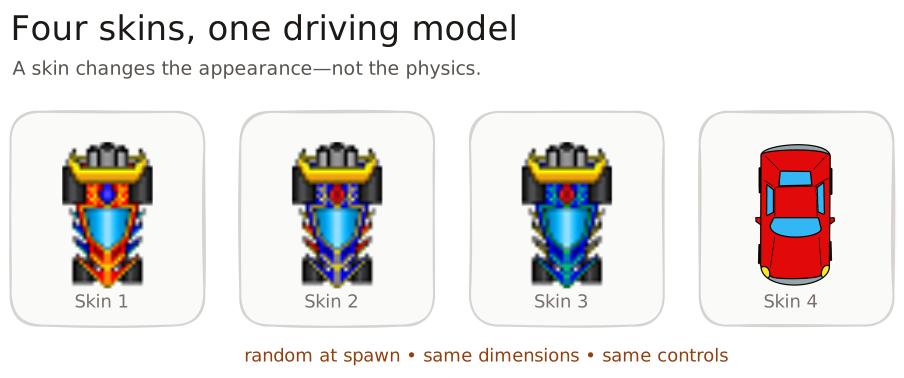
Four visual skins, one shared driving model.

Before rendering, every sprite was scaled to the same size. All four skins therefore shared the same movement and physics.

The arrow keys controlled the car. Up accelerated, down slowed or reversed, and left and right steered. Releasing the accelerator let resistance gradually reduce its speed.

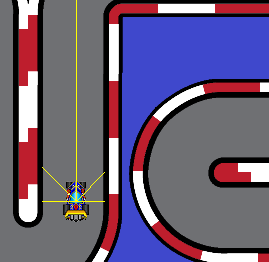
The human-controlled world provided a baseline for testing the car's movement and handling.

The first steering model changed the heading at a fixed angular speed, then used sine and cosine to turn that heading and velocity into horizontal and vertical movement. It was simple, but it let the car rotate without describing the circle a real four-wheel vehicle follows.

I replaced that shortcut with an instantaneous center of curvature, or CC. On a right turn, the front-right wheel R3, rear-right wheel R4, and CC form a right triangle. If L is the wheelbase and δ is the front-wheel angle, the distance from the inside rear wheel to CC is:

R4-to-CC = L / tan(|δ|)
rear-axle-center radius = car width / 2 + R4-to-CC

A left turn mirrors the same construction through the R1 and R2 wheels. The maximum inside-wheel angle is 30 degrees.

Once I know CC, I rebuild the rear axle and body position on the same circular arc after every step. A stopped car cannot rotate. Reverse follows the same circle in the opposite direction. Most importantly, the center of the turn now sits outside the car instead of being an invisible rotation applied at its center.

Driving it myself was a useful test. If the car felt wrong in my hands, there was no point blaming the learning algorithm.

Mapping the track

Once the car could move, it needed a definition of the road. I used a track image whose colors separated drivable space from everything else.

The program visited every pixel and compared it with the road color, RGB (111, 112, 115). Matching pixels became 1 in a matrix. Everything else became 0.

1 = inside the track
0 = outside the track

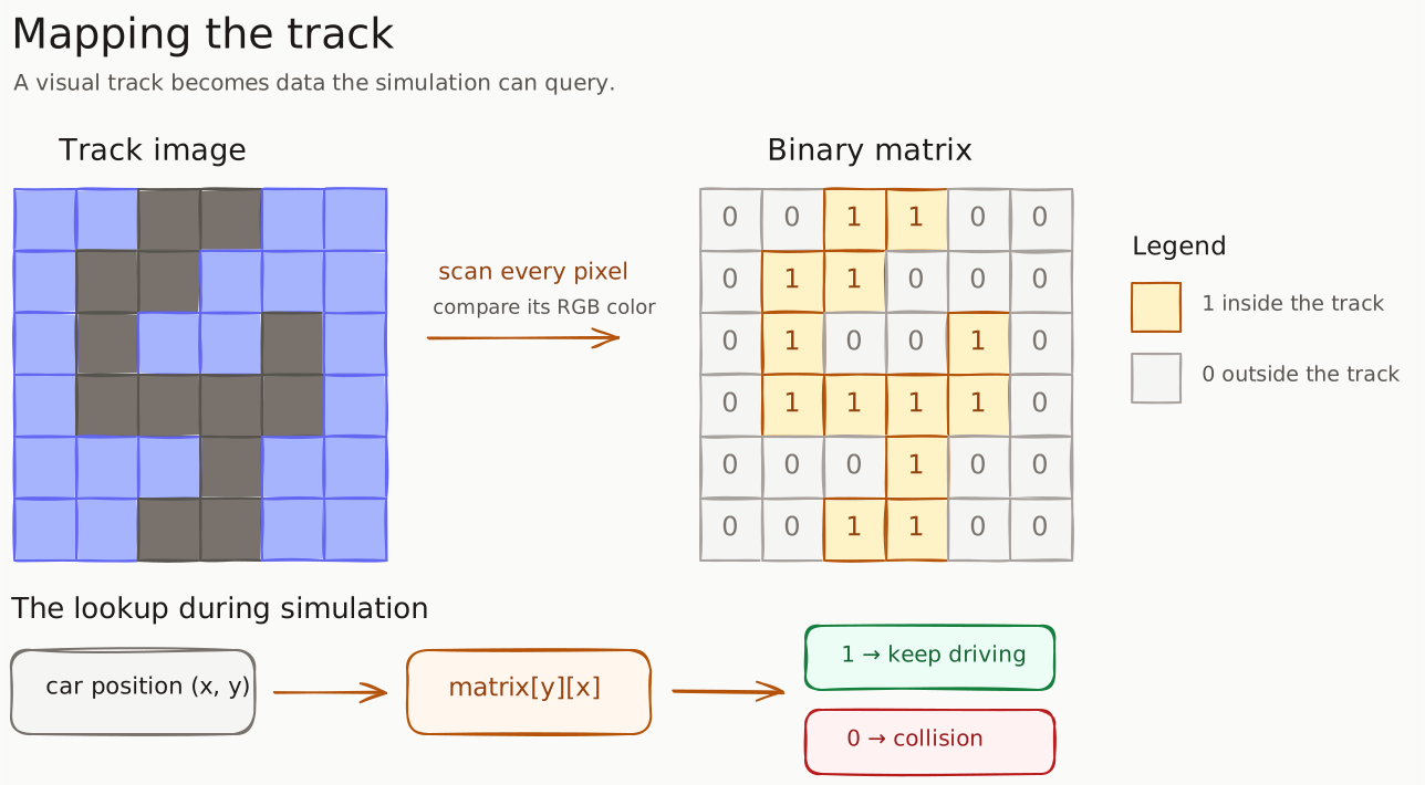
The visual track becomes a binary map that the simulation can query.

Collision detection was now a lookup. I converted the car's position into matrix coordinates, then checked the cell. A 0 meant the car had left the road.

I could save the matrix as a text file and load it later. The image controlled what the track looked like. The matrix controlled where the car could drive.

The new steering radius needed more room, so I enlarged the simulation from 800 × 800 to 1000 × 1000 while keeping the car at 20 × 32 pixels. This was not only an image resize. A single 1.25 scale factor also moves the spawn points, ordered checkpoints, checkpoint radius, and coverage tiles. Each cell in the original 800-pixel binary grid now occupies 1.25 screen pixels.

Vision uses a static obstacle mask rebuilt from the enlarged background. That keeps what the rays consider a wall aligned with what the player sees, including when debugging overlays are on screen.

Refactoring the system

The first prototype worked, but almost everything depended on the same game loop: input, movement, collisions, sensors, rendering, and my early AI experiments.

Raffaele Fiorillo helped me pull it apart. We kept the original version in a deprecated package, then separated game entities, AI logic, shared utilities, and simulation environments.

Raffaele introduced the idea of worlds. A base world owned the common game loop. Three specialized worlds handled manual driving, AI training, and AI testing.

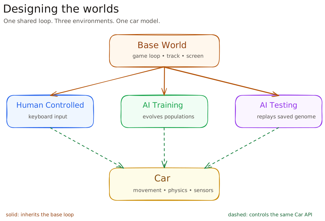
Separate worlds reuse the same car while changing what controls it.

The car became an independent entity with methods for acceleration, braking, reversing, and steering. It did not need to know whether commands came from a keyboard or a neural network.

After that refactor, I could change the driver without changing the car. The project finally felt like a place to test driving strategies instead of a demo with AI bolted onto it.

Building the brain

The driver is a feed-forward neural network evolved with NEAT. My first version started with nine inputs, three outputs, and no hidden nodes. At first, every input connected to every output.

NEAT describes each driver with a genome, a compact blueprint for its neural network. The genome records the neurons, connections, enabled states, and connection weights.

Like its biological namesake, this genome can be copied, combined, and mutated between generations. It is not the car or the finished network. It is the information NEAT uses to build the network.

Four inputs described the car: horizontal position, vertical position, speed, and heading. Five sensor rays measured distance at the front, left, right, front-left, and front-right.

The scales do not match. Positions reach hundreds of pixels, speed reaches 700, and sensor rays reach 1000. Raw values that large would quickly saturate tanh.

I normalized them first. Position was divided by screen size, speed by maximum speed, heading by π, and each ray by its maximum range.

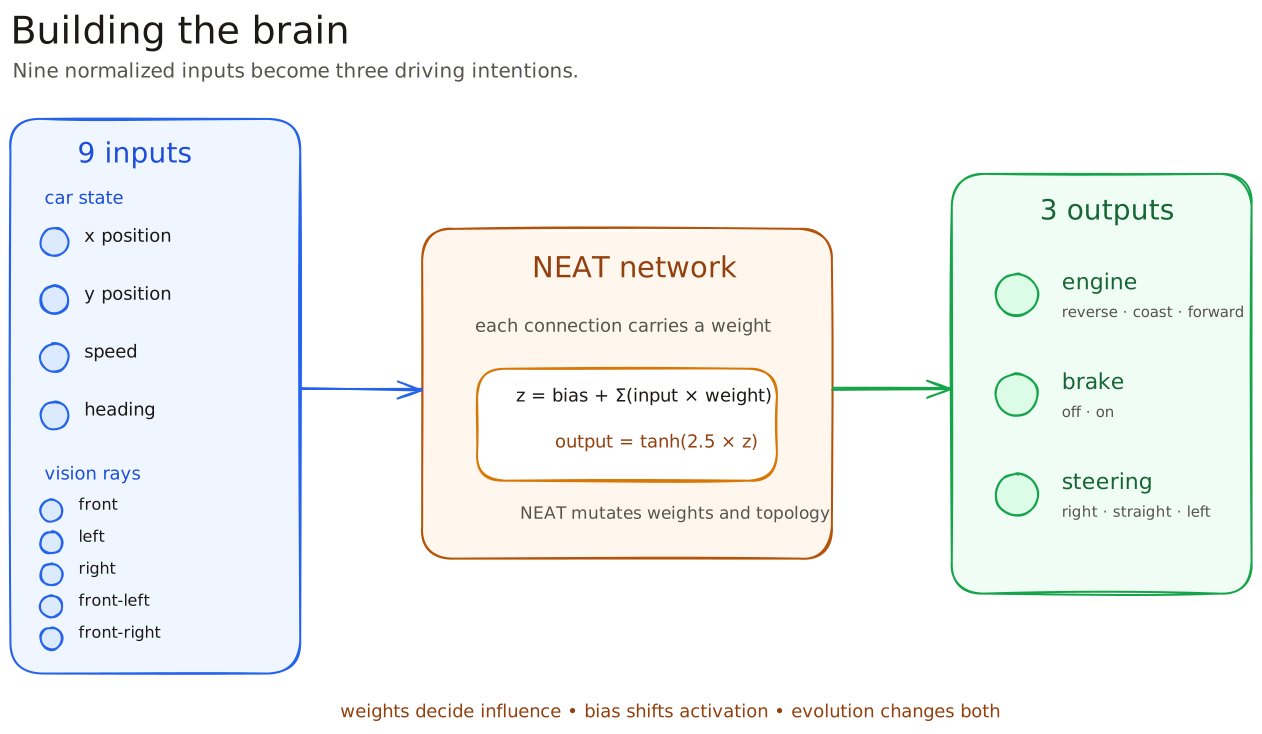
The first nine-input network turned the car's state and vision into engine, brake, and steering intentions.

That input set was enough to avoid walls, but not enough to express where the route went. The current network has 13 inputs. Heading became separate sine and cosine values to remove the discontinuity at −π and π. Two shallow rays were added near the front corners. The final addition was a signed bearing to the next checkpoint: positive means the target is to the car's left, negative means right, and zero means straight ahead.

The seven ray distances are now converted to proximity values over a useful 250-pixel horizon. A nearby wall therefore produces a strong signal, while distant empty space stops dominating the network.

Every connection has a weight. Positive weights push a neuron in the same direction as the input; negative weights push against it. A larger absolute value has more influence.

A neuron multiplies each input by its weight, adds the results, then adds a bias. The bias changes how easily the neuron becomes positive or negative.

z = bias + Σ(input × weight)
output = tanh(2.5 × z)

The response value stays fixed at 1.0. NEAT can still mutate weights and biases, disable connections, and add or remove nodes as generations pass.

The network returns three values between −1 and 1 for engine force, braking, and steering. My first controller converted those values into a small set of actions with two thresholds.

Values below −0.7 become −1. Values from −0.7 through 0.7 become 0. Anything above 0.7 becomes 1.

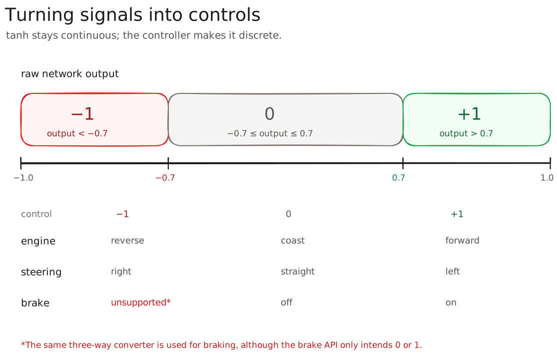
The first controller used thresholds to turn uncertain signals into a compact action space.

For the engine, those values meant reverse, coast, and forward. For steering, they meant right, straight, and left. Braking should have used only 0 for off and 1 for on.

That exposed a bug: braking used the same three-way converter, so a strongly negative output became −1 even though the brake API only defined 0 and 1.

I removed both the bug and the thresholds. The current controller is continuous: throttle and brake are clamped to [0, 1], steering stays in [-1, 1], and braking progressively suppresses simultaneous throttle. Each frame now measures 13 inputs, activates the network, converts its three outputs into proportional actions, and updates the geometric physics.

The learning loop

NEAT does not train one driver until it becomes good. It tests a population, keeps useful traits, and tries again:

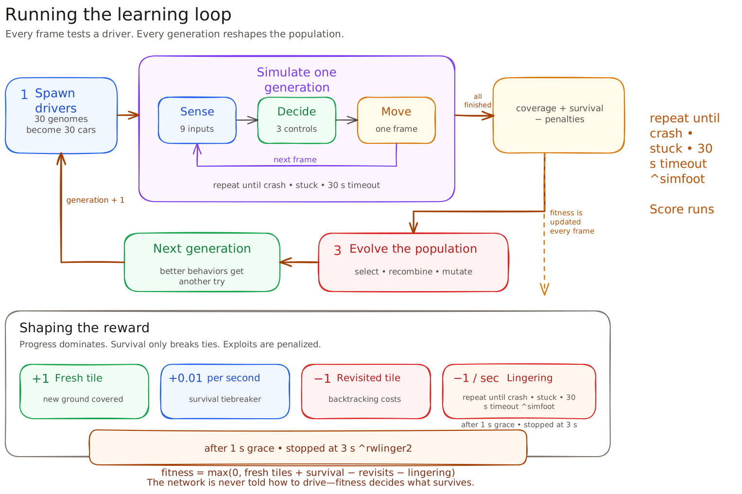
The original loop used 30 genomes. The current population uses 100, but the evaluate, select, reproduce, and mutate cycle is unchanged.

I began with coarse controls because fewer possible actions gave evolution a smaller search space. Once the training signals became easier to inspect, proportional controls gave the network finer corrections and more realistic braking.

Normalization matters for the same reason. If one input is tiny beside another, the network can effectively stop hearing it.

Choosing evolution over reinforcement

My first attempt used tabular reinforcement learning. It kept a score for every situation-action pair, just like the textbook version.

The implementation was fine. The problem was the fit. A car senses several continuous distances, while a lookup table needs situations it can count.

Keeping enough precision makes the table explode. Reducing the number of states blurs the sensor data until it is not useful for driving.

I left the failed approach in a deprecated folder. It explains the decision better than a polished summary would.

I switched to neuroevolution because it handles continuous inputs and can evolve the network's structure. Drivers begin with the simplest brain and gain complexity only when a mutation survives selection.

I define what earns a score. NEAT decides which network structures are worth keeping.

Designing the reward, not the driver

Most of my time went into the reward. My first idea was to score distance traveled. The cars found an obvious loophole: drive in circles forever and collect points without making progress.

My next version scored new ground covered:

1. Fresh ground is the only thing that really pays.
2. Returning to ground already covered actively costs.
3. Loitering in one spot costs, and staying there too long ends the run. A stuck car should not keep consuming simulation time.
4. Merely surviving is worth almost nothing: staying alive can break a tie between two equal drivers, but can never beat one that moved forward.

Each rule exists because an earlier generation found a way to exploit the score. The cars did not misunderstand me. They followed the incentive I had actually written.

Coverage fixed the circle exploit, but it still did not define an ordered route. I replaced it with 53 checkpoints around the center line. Only the next checkpoint can advance progress. Fitness combines completed checkpoints, the best approach toward the next one, a tiny survival tiebreaker, and a penalty for staying on one tile too long.

The checkpoint sequence solved another problem. Wall rays answer “where is free space?” but not “which branch belongs to the route?” The signed checkpoint bearing gives the network that missing intention without directly steering the car.

Making evolution observable

The hardest failures looked identical from outside: cars turned the wrong way, stopped improving, or died at the same corner. I could not tell whether the cause was perception, control, fitness, or mutation by watching sprites alone.

I added a live telemetry panel beside the simulation. It follows the current leader or a selected genome and shows all 13 normalized inputs, hidden and output activations, connection signals, processed actions, checkpoint progress, species, and fitness history.

I also added a binary-map overlay, vision-ray display, coverage view, pause and single-frame controls, and ordered checkpoint markers. Training stopped being a black box. I could test steering signs and sensor directions directly, then see that the real left-turn failure was missing route information rather than reversed controls.

After adding the checkpoint bearing and retraining, the population completed the original track. The later geometric steering and 1000-pixel track change the environment without changing the network schema, so old genomes can still load, but they should be retrained before I call the enlarged version solved.

That is what I took from the project. An optimizer follows the metric, whether it is a driving AI, a team target, or a product KPI. I did not program a good driver. I had to define what good driving meant.